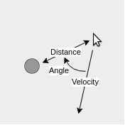
Your mouse controls a robot in a flat plane, and you want to know its location. Unfortunatley, the robot is in an almost entirely empty space that provides very little information that can be used to localize. The only usable feature in your environment is a pillar near its center. With your robot's sensors, you can determine the following information at any point in time:
Of course, data is never exact; not even in this simulation. For us, this means a hardcoded localization algorithm (perhaps using trigonometry) would not necessarily be effective. In addition, one could easily imagine more and more complex scenarios, where hardcoded algorithms would quickly become intractable. In order to localize the robot under these conditions, we will use a particle filter.
Particle filters are a class of tools used to estimate the state of something with limited and/or incomplete measurements that contain random noise. In order to understand how particle filters work, we first have to describe what a "particle" is. Also known as a sample, a particle is really just a guess at what the state we're trying to describe could be. For example, if we knew we were in downtown Ann Arbor, but didn't know our exact location, an individual particle could be the intersection of Main Street and Liberty. Another particle could be the intersection between Ashley and Huron. And so on.
With a large enough number of particles, it's likely that at least one will be close to the truth. At this point, the process is iterative. Each time we receive a new batch of information, the particle filter evaluates how well each particle fits the data, and creates a new set of particles primarily located near the best from the previous iteration. By repeating this process over and over, the particle filter can build a belief of what the state actually is.
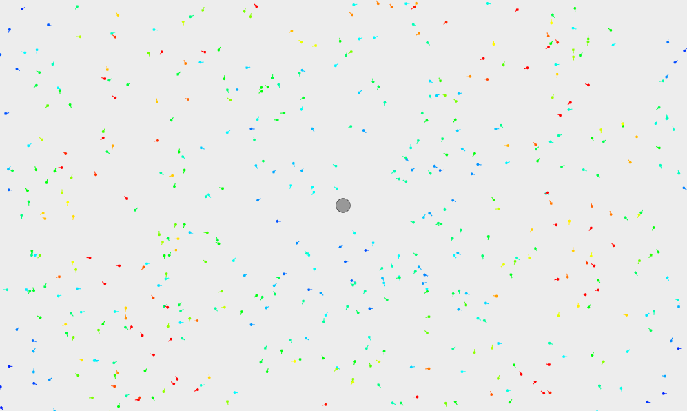
1. Initialization of Particles
To start out, the algorithm randomly places a large number of particles in the state space, that is, all possible locations of the robot. Because there are a large number of particles, seeding them randomly ensures a relatively even distribution across the state space, and that there will be particles near the true location of the robot.
2. Get Robot Measurements
Each iteration of the algorithm starts out with data that is received from the robot. In our case, we recieve 3 pieces of information -- the robot's velocity, the heading to the pillar, and the distance to the pillar.
3. Weight Particles
Based on the information we know about the robot, we can assign each particle a "weight" based on how well it matches with the robot's data. A higher weight means the particle is a closer match. This is indicated on the display by the color of the particle; blue represents a low weight, up to red which represents a high weight.
4. Predict Robot Location
By averaging the location of all the particles with higher-than-average weights, the particle filter approximates the location of the robot.
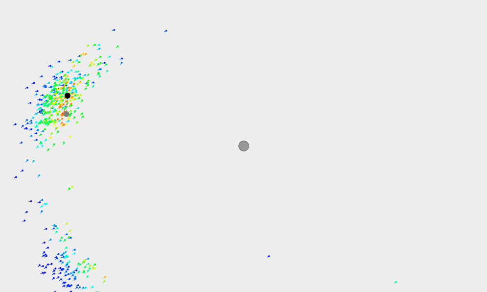
5. Resample Particles
The algorithm randomly distributes the next set of particles at the locations of the previous set, with most of the new particles being put by the old particles with the highest weights. In addition, a small percentage of the particles are randomly seeded throughout the world, in case the robot isn't near any of the current particles.
6. Translate Particles
Since we have an estimate of the robot's velocity, the particle filter translates each particle by the expected distance that the robot has moved. In addition, we add noise to both how far the particle travels and which way it travels, in recognition of the fact that the robot's velocity is not necessarily 100% accurate.
7. Return to Step 2 and Repeat